
Autonomous driving using three simple vision algorithms
The purpose of this post is to familiarize the reader with three vision algorithms used for a simple autonomous driving algorithm.
Autonomous driving is a very complicated subject. To make a car drive fully autonomously, big neural networks, machine learning and a lot of engineering needs to be applied. A very rudamentary autonomous driving algorithm can be created using three vision algorithms described in this post. The efficiency of this approach is very low, but it does not require any knowledge of artificial intelligence to be used.
The goal of the algorithm is to drive along the road and control the speed accordingly to curves ahead. To see the algorithm in action an environment is going to be needed. Since testing in real world is expensive, complicated and probably illegal, a virtual environment is going to be used. There is a lot to choose from: Carla, AirSim, or any other driving game that has basic programming support, like GTAV with ScriptHook or Live for speed.
Since the purpose of this blog entry is to focus on autonomous driving, obvious parts of the application are skipped (screen grabbing, simulation parameters reading and control override). You can look it up in the source here: AutoCruise.
The algorithm workflow uses three vision algorithms stacked on eachother: Perspective, Sobel and finally Sliding window.
Perspective
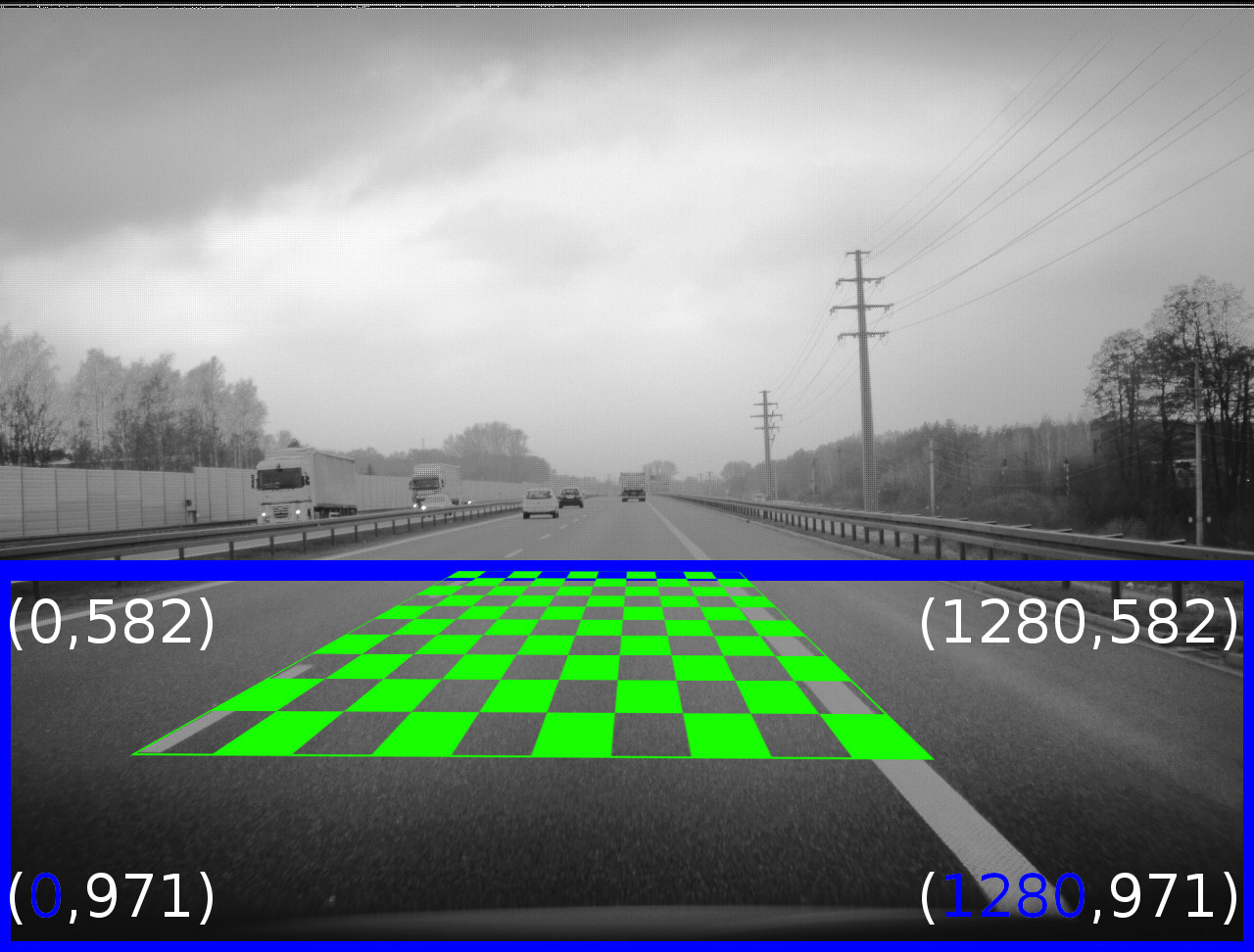
First algorithm used in the workflow is perspective transformation. It creates a birds-eye view from drivers point of view. The purpose of it is that it is far easier to find road edges and lanes as they will be parallel instead of converging to the vanishing point.
The perspective transformation is a 3D transformation of the view pane, such that lower parts of the image will be put farther from observer point of view, while the upper parts will be closer.
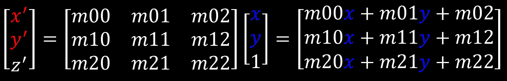
Such transformation can be achieved by creating transformation matrix manually or use FindHomography() function from opencv library. Using the second approach, the lower part of input image needs to be squeezed to counter the perspective projection of 3D world to 2D pane viewed from driver point of view:
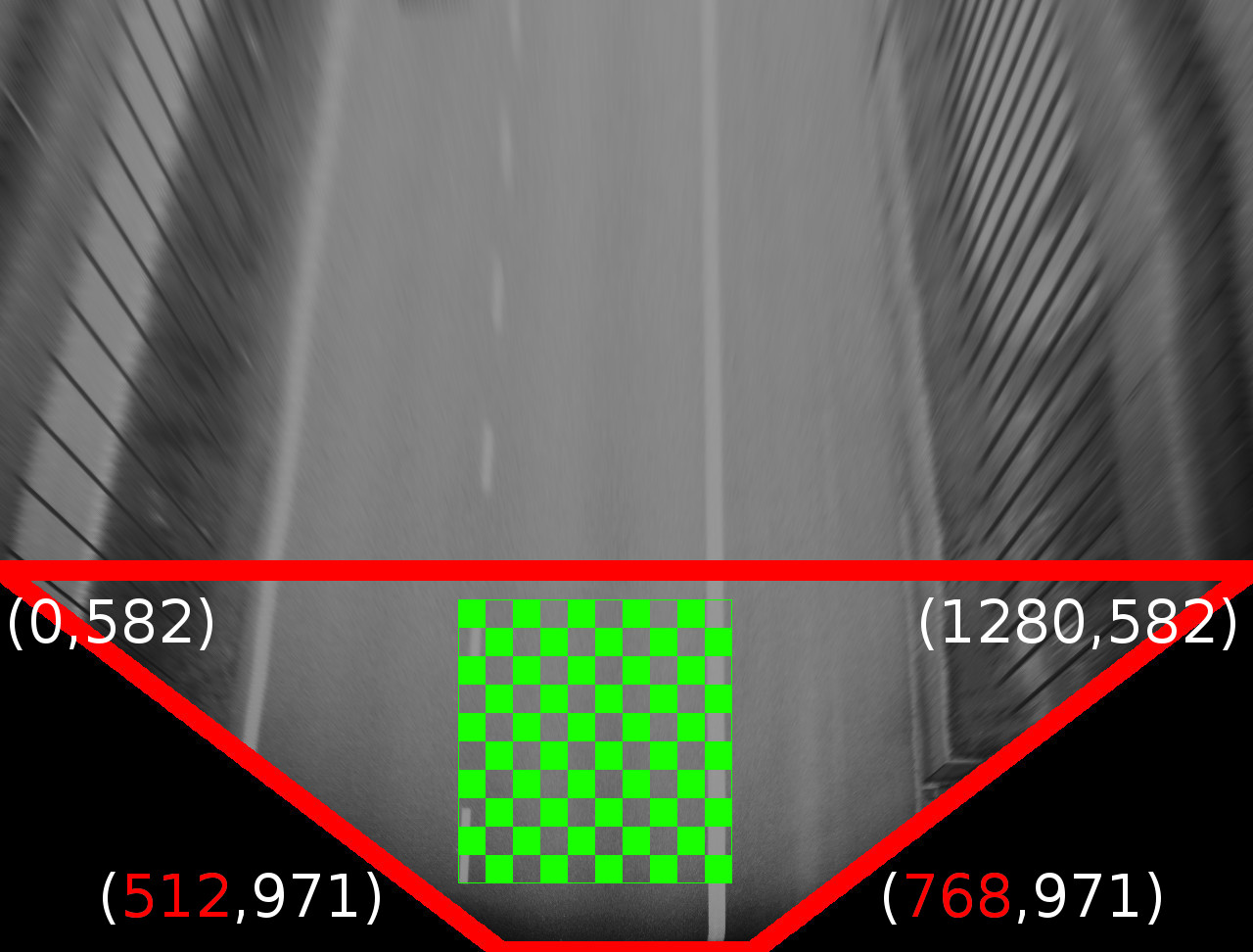
With transformation matrix returned from FindHomography() new position of each pixel can be calculated from source image:
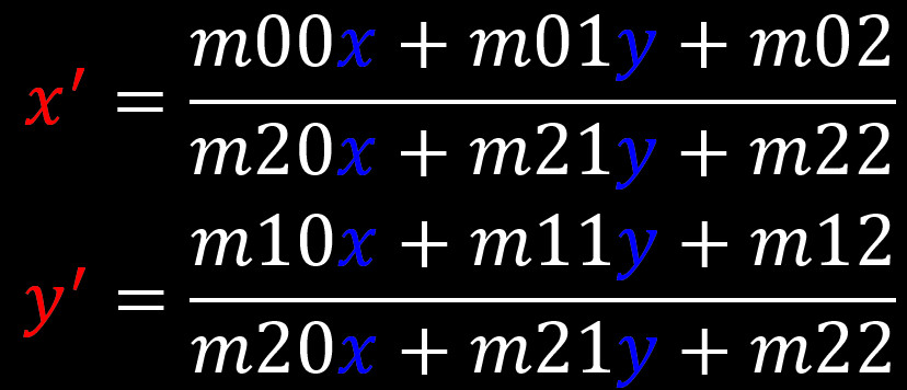
…or simply use opencv WarpPerspective() function, thus creating a perspective transformed image.
Sobel
The perspective transformed image is fed to next algorithm in workflow: an edge finding algorithm, Sobel. Its purpose is to highlight image edges that should be “interesting and meaningful” for driving algorithm. It will highlight image edges that distinguish themselves in x-axis in comparison to background noise.
For learning purposes, the focus will be put on part of the image where a clear lane marking can be seen. Note that we are working on grey image, so each pixel is represented as 8-bit value with range from 0 to 255.
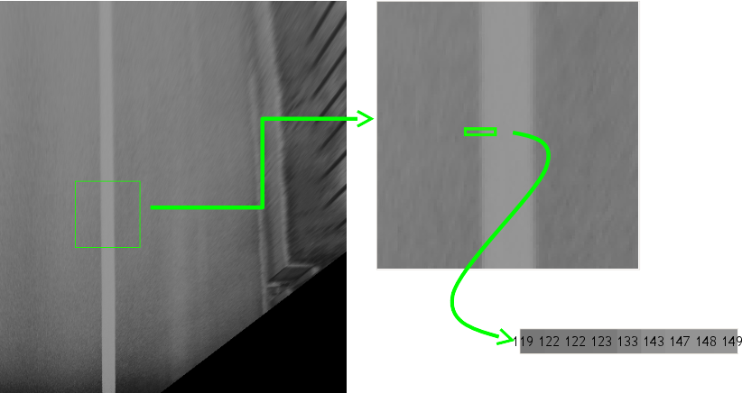
It can be clearly seen that values go up from 119 to 149. Sobel algorithm transforms the image by comparing each pixels value to its right neighbor, therefor creating a difference map in form of an image which contains result of subtracting each pixels value to its right neighbor. Since the difference can be positive as well as negative, the result of subtraction is added to 128 (perfect grey color) so that the edge will be brighter if right neighbor pixel was brighter and darker edge in other case.
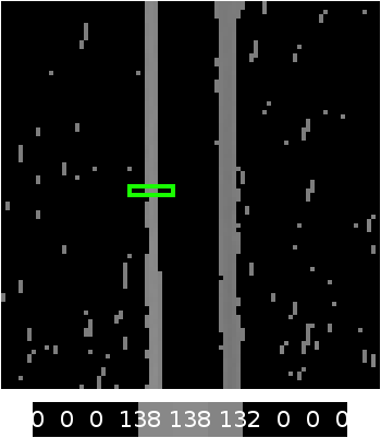
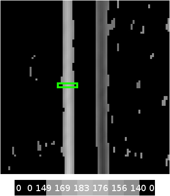
To increase effectiveness of highlighting distinguished image edges a parameter called kernel has been introduced which compares a set of pixels to neighboring set of pixels in form of rectangle with side length of the kernel. This operation results in image that contains only edges that are highly distinguishable.
Sliding window algorithm
The last vision algorithm used in the workflow is Sliding window algorithm. Its purpose is to track image edges that are highly likely the road edges. This algorithm is quite resistant to image noise but not that accurate - just enough for purpose of a simple autonomous driving algorithm.
Starting point of the Sliding window algorithm is placing a search window (of preconfigured size) in place where a lane should be present: the front end corner of the car. Next, the window is slidden upwards along the most distinguishable edge. Every time the window is moved upwards (by its height size) from its last position, a new horizontal position is calculated by weighted average on x-axis: the more pixels (with bigger values) are found on horizontal position inside the window, the more windows new position will be close to this position (in x-axis). Repeat this until the search window goes out of bounds of the image.

After both left and right sliding windows have been moved to the upper boundaries of the input image, two paths have been created which should represent the road edges.
Driving algorithm
With the (probable) road edges found, a rudamentary driving algorithm is used: keep a steady 50kmh speed and slow down proportionally to lane curvature and steer to keep the car between the lanes. Driving precisely between the found lane edges needs to include steering parallelly to them. This needs a lot of experiments to dial steering right if done manually. To make most out of this approach, machine learning should be used with pre-recorded driving data. This way the algorithm should be able to clone the recorded driving style, but that is a topic for another blog entry.
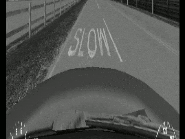
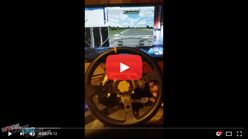
The final result looks like this:
Software developer, Drift racing driver
LinkedIn: Tomasz Sułkowski